Lab 02: Flow Around Cylinders

Experiment Overview

The cylinder is one of the most studied shapes in fluid mechanics because it captures bluff-body aerodynamics in a clean, symmetric geometry: stagnation, attached flow, boundary layer separation, and a turbulent wake. Understanding how pressure distributes around a blunt body — and how drag arises from that distribution — is directly relevant to designing fuselages, struts, landing gear, and external fuel tanks.

• Measure the full surface pressure distribution around a cylinder at two speeds: 10 m/s (Re ≈ 23,500) and 15 m/s (Re ≈ 35,300)
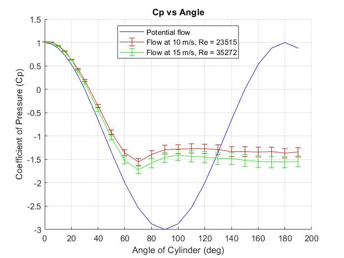
• Compute the pressure coefficient C_p at each angular position and compare against ideal potential-flow theory
• Numerically integrate the pressure distribution to extract the drag coefficient C_d
• Observe how increasing Reynolds number delays flow separation from the cylinder surface

Equipment & Tools

• ERAU open-circuit wind tunnel
• 1.4-inch aluminum cylinder with single static pressure port (24 angular positions, 0°–180°)
• Differential pressure transducer and analog manometer
• Angular rotation fixture for cylinder positioning
• MATLAB for data acquisition, coefficient computation, and plotting

Approach & Key Equations

A 1.4-inch cylinder with a single static pressure port was rotated to 24 angular positions from 0° to 180°, capturing differential pressure at each angle for both test speeds. The pressure coefficient was found by normalizing each reading against the freestream dynamic pressure. Potential flow theory predicts C_p = 1 − 4sin²(θ), which was plotted alongside measured data for comparison.

Drag was extracted by integrating C_p·cos(θ) around the cylinder using MATLAB’s trapz function. This pressure-integration method converts the mapped surface pressures directly into a net streamwise force coefficient, requiring no physical force sensor:

C_d = ∫₀^π C_p cos(θ) dθ

Key Results

• Below ~40°, experimental C_p closely matched potential flow near the stagnation point. Past ~40°, the measured pressure deviated sharply — the viscous boundary layer separated and the inviscid model no longer applied.
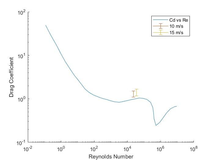
• Both tests were subcritical (Re < 300,000): no drag crisis occurred and flow separated on the upstream portion of the cylinder at both speeds.
• At 15 m/s, flow remained attached slightly longer than at 10 m/s — a direct demonstration that higher Reynolds number delays separation, reducing the low-pressure wake region.
• C_d = 1.31 at 10 m/s and C_d = 1.42 at 15 m/s — drag coefficient increased with speed because a wider turbulent wake raised the pressure drag contribution.

MATLAB Code

Pressure data was loaded from 24 .mat files per test speed, converted to Pascals, and integrated to produce C_p and C_d. The potential flow reference was computed analytically for comparison.

% Pressure coefficient at 10 m/s
Cp_10 = dp_10ms / (0.5 * density * 10^2) + 1;

% Potential flow reference
Cp_potential = 1 - 4 .* sind(angles).^2;

% Drag coefficient via trapezoidal integration
theta = deg2rad(angles);
Cd_10 = trapz(theta, Cp_10 .* cos(theta));  % = 1.3055

Valuable Takeaways

• Inviscid theory breaks down exactly where it matters most — at separation. The agreement near stagnation and divergence past 40° shows precisely where viscosity enters the picture, a boundary that governs drag on every real bluff body.
• Drag can be extracted entirely from surface pressure data via integration, without a force balance. This method is used in wind tunnel testing and CFD validation to decompose drag into pressure and viscous components.
• Reynolds number controls separation. Even the modest difference between 10 and 15 m/s produced measurable differences in flow attachment — reinforcing why scale effects must be considered when interpreting wind tunnel data for full-size aircraft.
• Developed practical skills in angular pressure acquisition, numerical integration of surface distributions, and structured comparison of experimental versus analytical aerodynamic predictions.